5 Analysis

The analysis of the results was conducted in two main ways. First it was important to analyze the aggregation function. One concern with the aggregation procedure herein used is that it is not possible to provide a formula which describes explicitly how individual characteristics affect the final level of democracy (Gründler & Krieger, 2021). Hence, the aggregation cannot be justified by theoretical assumptions (Gründler & Krieger, 2021). This is gap that this contribution attempted to fill. To do that it compared the aggregation method applied here to an already existing and established aggregation method.

In that effort the index that served as baseline of comparison was the EDI (Coppedge, Gerring, Knutsen, Lindberg, Teorell, Alizada, et al., 2021). There were many reasons for this. For one, as mentioned previously, the breadth of data made available in the V-Dem dataset can hardly be overstated. It contains more than 4000 variables for more than 200 countries from 1789 to 2020 (Coppedge, Gerring, Knutsen, Lindberg, Teorell, Alizada, et al., 2021). Furthermore, the selection and construction of regime characteristics is theoretically well grounded, each rating is given a confidence interval, the raw data is publicly available, and its codebook clearly describe coding and aggregation methods (Coppedge, Gerring, Knutsen, Lindberg, Teorell, Altman, et al., 2021; Coppedge, Gerring, Knutsen, Lindberg, Teorell, Marquardt, et al., 2021; Gründler & Krieger, 2021). Lastly, the EDI employs a combination of most traditional forms of aggregation (Coppedge, Gerring, Knutsen, Lindberg, Teorell, Altman, et al., 2021; Coppedge, Gerring, Knutsen, Lindberg, Teorell, Marquardt, et al., 2021; Gründler & Krieger, 2021).

The second step was to compare the results herein developed, not only with the already existing SVMDI index, but with their different breadths of Merkel’s (2004) concept of Embedded Democracy. This was an effort to conclude to what extent can an SVM based democratic index with broader concepts of democracy effectively identify gradations of democracy. Since there is no simple objective way to measure it, this contribution analyzed specific cases, which could indicate strengths and weaknesses of the different variations.

5.1 Aggregation

The EDI is composed of five mid-level composite indicators, three of them are measures taken from various sub-indicators and aggregated by a Bayesian Factor Analysis Model (BFAM), one manually coded measure, and one objective measure (Coppedge, Gerring, Knutsen, Lindberg, Teorell, Altman, et al., 2021; Coppedge, Gerring, Knutsen, Lindberg, Teorell, Marquardt, et al., 2021). These were described further as they constitute the variables used for both the EDI and the SVM index. Since the main issue the SVM index was attempting to address was the unknowable aggregation function, no composite index was used, but rather their subindices. The reason for this was simple. These composite indices are themselves aggregated. If the objective was for the SVM to decide how to aggregate variables and to then compare the aggregation results with the EDI, then it was important to use the lowest level variables available.

The first of the aggregated indices measures freedom of association (v2x_frassoc_thick) (Coppedge, Gerring, Knutsen, Lindberg, Teorell, Altman, et al., 2021). It is itself composed of six low-level indicators, i.e. party ban (v2psparban), barriers to parties (v2psbars), opposition parties autonomy (v2psoppaut), elections multiparty (v2elmulpar), Civil society organization (CSO) entry and exit (v2cseeorgs) and CSO repression (v2csreprss) (Coppedge, Gerring, Knutsen, Lindberg, Teorell, Altman, et al., 2021). CSOs are considered “interest groups, labor unions, religiously inspired organizations (if they are engaged in civic or political activities), social movements, professional associations, and classic non-governmental organizations (NGOs), but not businesses, political parties, government agencies, or religious organizations that are primarily focused on spiritual practices” (Coppedge, Gerring, Knutsen, Lindberg, Teorell, Altman, et al., 2021, p. 192).

The second aggregated index measures clean, free, and fair elections (v2xel_frefair) (Coppedge, Gerring, Knutsen, Lindberg, Teorell, Altman, et al., 2021). It is composed of eight low-level indices, i.e. Election Management Body (EMB) autonomy (v2elembaut), EMB capacity (v2elembcap), election voter registry (v2elrgstry), election vote buying (v2elvotbuy), election other voting irregularities (v2elirreg), election government intimidation (v2elintim), non-state electoral violence (v2elpeace), and election free and fair (v2elfrfair) (Coppedge, Gerring, Knutsen, Lindberg, Teorell, Altman, et al., 2021). It is important to mention at this point that many of the characteristic that relate to elections in these two composite indices were only available during election years and if there was an electoral regime to speak of (v2x_elecreg). Those characteristics were modified so that the data repeated itself in the years in between elections, as recommended by V-Dem’s codebook (Coppedge, Gerring, Knutsen, Lindberg, Teorell, Altman, et al., 2021). Furthermore, should an election data be missing in the first year of analysis, the data was backfilled with the most recent value, as V-Dem does with the US and the UK (Coppedge, Gerring, Knutsen, Lindberg, Teorell, Altman, et al., 2021).

The third aggregated index measures freedom of expression and alternative sources of information (v2x_freexp_altinf) (Coppedge, Gerring, Knutsen, Lindberg, Teorell, Altman, et al., 2021). It is composed of 9 low-level indicators, i.e. media censorship effort (v2mecenefm), harassment of journalists (v2meharjrn), media bias (v2mebias), media self-censorship (v2meslfcen), print/broadcast media critical (v2mecrit), and print/broadcast media perspectives (v2merange), freedom of discussion for men (v2cldiscm), freedom of discussion for women (v2cldiscw) and freedom of academic and cultural expression (v2clacfree) (Coppedge, Gerring, Knutsen, Lindberg, Teorell, Altman, et al., 2021).

The last non-objective indicator measures whether the chief executive and the legislature are elected, directly or indirectly, through popular elections (v2x_elecoff). This indicator is a manually coded, expert-based indicator. It is very minimally defined and only explicates whether there are elections for the aforementioned high offices or not. Some elections that one could call controversial are still counted in this indicator (Coppedge, Gerring, Knutsen, Lindberg, Teorell, Altman, et al., 2021).

The last indicator measures the degree of suffrage within the populace (v2x_suffr) (Coppedge, Gerring, Knutsen, Lindberg, Teorell, Altman, et al., 2021). It is objective, composed of factual indicators and provides the share of the adult population that is granted suffrage. This only encompasses de jure suffrage, not de facto. This means that it does not take into consideration restrictions based on age, residence, criminal record, or legal incompetence (Coppedge, Gerring, Knutsen, Lindberg, Teorell, Altman, et al., 2021).

These indicators are aggregated in three steps. First, they are aggregated into a multiplicative indicator (Coppedge, Gerring, Knutsen, Lindberg, Teorell, Altman, et al., 2021; Coppedge, Gerring, Knutsen, Lindberg, Teorell, Marquardt, et al., 2021). All values are multiplied equally. Second, they are aggregated into a weighted additive index. The BFAM aggregated indices are multiplied by 0.25, while the other two are multiplied by 0.125, which is supposed to penalize the latter (Coppedge, Gerring, Knutsen, Lindberg, Teorell, Altman, et al., 2021; Coppedge, Gerring, Knutsen, Lindberg, Teorell, Marquardt, et al., 2021). “The additive part of the formula lets the two components that can achieve high scores based on the fulfillment of formal institutional criteria (elected officials and suffrage) together weigh half as much as the other components that enjoy a stronger independent standing in terms of respect for democratic rights (clean elections, freedom of organization and expression)” (Coppedge, Gerring, Knutsen, Lindberg, Teorell, Marquardt, et al., 2021, p. 5). An average is then taken of the two indices to form the final EDI (Coppedge, Gerring, Knutsen, Lindberg, Teorell, Altman, et al., 2021; Coppedge, Gerring, Knutsen, Lindberg, Teorell, Marquardt, et al., 2021).

The SVM index, on the other hand, used the low-level indices without aggregating them into mid-level indices. They were, hence, considered as individual variables. However, due to the coding rules for some of them, a fair amount of the data had to be adapted. For starters, to be able to track different country-year observations reliably, a form of code had to be used to identify each country. Country names are not ideal in that effort, since names can change over time or a country might dissolve into multiple entities, e.g. Germany, Czechoslovakia, Vietnam (Coppedge, Gerring, Knutsen, Lindberg, Teorell, Alizada, et al., 2021). To address this issue, this contribution made use of the ISO 3166-1 Alpha-3 standard (International Organization for Standardization [ISO], 2021). For countries that no longer exist as formal entities, e.g. the German Democratic Republic, their historic codes were used (ISO, 2021). These were then combined with the variable related to the year in question to create individual identifiers. Furthermore, one could assume to make the coding of variable less cumbersome, some expert-based variables are coded in the V-Dem dataset as missing based on other expert-based variables. For instance, the autonomy of opposition parties (v2psoppaut) is generally only coded if the barriers to forming parties (v2psbars) are not so restrictive as to not allow non-government affiliated parties to form. The same is true for many electoral variables. Unless there are elections, they are not at times coded. If all of those observations were removed, many countries in the lower end of the spectrum would be excluded from the dataset. To compensate for this, such variables were given the lowest possible score, as that relates to the intent of not coding them (Coppedge, Gerring, Knutsen, Lindberg, Teorell, Altman, et al., 2021).

A further, yet minor problem, is that about 0.03% of the datapoints in the observations were missing, hence there were minor gaps in the data. To deal with this issue and avoid the removal of entire observations due to occasional minor gaps, cubic spline interpolation was used to fill them. This technique is often used for such purposes (Coppedge, Gerring, Knutsen, Lindberg, Teorell, Alizada, et al., 2021; Gründler & Krieger, 2021). The objective here was to calculate a function that best described the points in a dataset by finding the polynomial of the lowest possible degree and utilize that to fill gaps in the data (Korstanje, 2021). While in a large scale that would skew the data, a minimal amount of the dataset was interpolated and hence shouldn’t have a substantial effect.

Taken that into account, the final dataset had 16390 observations, and the priming data had 4616. The priming data, as described in Section 3, was used to train the dataset and then it calculated the index for each observation in the total dataset 2000 times. The final index was then extracted by taking the median of all iterations for each observation.

Figure 1 - Distribution between EDI and the SVM Index

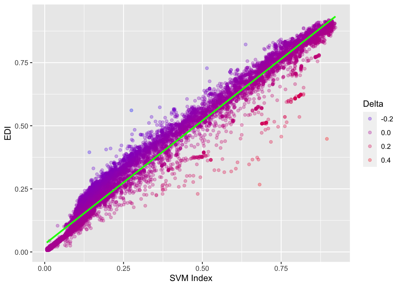
These SVM results were then compared with the original EDI. An additional variable was created by calculating the delta between both indices. As shown by Figure 1 and as expected, the two indices correlated substantially, particularly in the extremes of the spectrum. This was expected as there was little disagreement on the top and bottom ends of the scale, as mentioned previously (Cheibub et al., 2010; Gründler & Krieger, 2021; Lindberg et al., 2014). An example of this dynamic is, as Figure 2 shows, Germany, as it relates to the ISO 3611-1 Alpha 3 code “DEU”. This does not include, for instance, the German Democratic Republic, i.e. “DDR” (ISO, 2021). Throughout its modern history, Germany has inhabited both ends of the democracy-autocracy spectrum. Hence, it exemplified the similarity between indices in the extremes of the scale. However, there were minor discrepancies in its middle section. Overall, no country averaged a difference in score of more than a decile. Out of those, the majority had a higher EDI than SVM index.

Figure 2 - Index development over time for Germany

In the interest of pinpointing which variables might have played a role in the disparity between the two indices, the observations that diverged by more than 0.01 were analyzed separately. An OLS regression, evidenced on Table 2, showed both expected and insightful results. The correlation between the variables and the indices was noticeable and statistically relevant. This was obviously to be expected as both indices were made up of said variables. The sole exception was the influence of media bias and media self-censorship on the EDI, which were not statistically relevant. The models for both indices were themselves statistically relevant and explained a very high degree of the indicators’ variance, again also expectedly.

Table 2 - OLS Regression for EDI and SVM Ind.

Notes: Table created using the stargazer function (Hlavac, 2022).

The model for the EDI explained an even higher degree of its variance than the one for the SVM Index, which indicated that the adaptations introduced to the dataset did not have a sizeable effect in the relationship between the variables and the index. One would expect that, should the adaptations have had a big impact on said relationship, that the index composed directly of those variables, i.e. the SVM index, would have a higher degree of variance explained by them. That was, however, not the case, albeit by a very slim margin¹⁰.

More interestingly for the purposes of this contribution was the effect that individual variables had on the individual indices. In the SVM index no variable had an effect on the dependent variable larger than nine hundredths of the scale. The two variables with the largest effect were, in decreasing order, presence of elected officials (v2x_elecoff) and share of population with suffrage (v2x_suffr). This makes sense from a theoretical standpoint. These two characteristics are generally accepted as necessary conditions for a democratic regime (Coppedge, Gerring, Knutsen, Lindberg, Teorell, Marquardt, et al., 2021; Dahl, 1989; Gründler & Krieger, 2021; Merkel, 2004). However, they were but two of 15 variables that also had an effect in the hundredth range.

A similar dynamic played out with the EDI, but with key differences. The effect of nearly all variables ranged from the thousandth to the hundredth range. Much like the SVM index, the same variables in the same descending order, i.e. v2x_elecoff and v2x_suffr, were the source of the highest degrees of variance. However, unlike the SVM index, these were the only variables that had an effect in the tenth range. Furthermore, apart from two other variables, i.e. v2merange and v2cldiscw, all other variables had a similar or lower influence on the variance of the EDI in comparison to the SVM index.

This indicated that, despite the efforts to penalize v2x_elecoff and v2x_suffr in the additive index, these two variables still exert a big influence on the overall EDI due to the multiplicative index. While it’s important that these variables play a big role in assessing the level of democracy, they often undermine the remaining characteristics. This was further exemplified by cases such as Russia and Colombia. These cases were chosen because they undergone considerable movement in the middle part of the spectrum. Furthermore, they were good examples of different ways the disparate aggregation between the indices might have affected the results.

Figure 3 - Index development over time for Russia

Figure 4 - Development of mid-level variables for Russia

Russia, for instance, as shown in Figure 3, differed most noticeably between 1919 and 1937 and after 1999. During the first period the value of the SVM index laid below 0.1 whereas the EDI laid above that value. In fact, the former stayed below the latter all the way up to the early 1990s. After 1999 the SVM index dropped more pronouncedly than the EDI. The discrepancy in the early 20th century, considering the information of the OLS regression, it could be argued, could be attributed to the high levels of suffrage in this period. Figure 4 shows the development of the individual categories that compose the EDI over time. These categories were composed of the average centralized value of the low-level indices for each corresponding mid-level index. While said figure did not allow for the comparison of their specific values with each other, they did allow one to attempt to identify which of the categories might have had an effect on the overall index. Indeed, while the aggregated indices had a larger effect on the SVM index, the EDI was propped up by the high level of suffrage. Throughout the 20th century the SVM index seems to have been particularly sensitive to the v2xel_frefair category, which relates to free and fair elections. The variation of the SVM index in both the 1930s and 1990s was an indication of that. However, this dynamic was further evidenced by the development of the categories post 1999. While v2x_elecoff and v2x_suffr, which are not aggregated using a BFAM on low-level indices, remain relatively high, the other three aggregated categories all decrease in that period, which led to a much steeper curve in the SVM index.

Figure 5 - Index development over time for Colombia

Figure 6 - Development of mid-level variables for Colombia

Colombia was a further example, though the dynamics of its development were slightly different than Russia’s. As Figure 5 indicates, there was no period in which the SVM index went above the EDI. In fact, the SVM index was consistently and considerably below the EDI. However, both followed relatively similar patterns. This showed that both are similarly susceptible to the variation in the individual categories, as indicated by Figure 6. The difference laid in the relatively high levels of the v2x_elecoff variable throughout this period. The closest the two indices come to each other was during the mid-1950s where there was a steep drop-off in the v2x_elecoff and a middling v2x_suffr variable. However, when both of them rose simultaneously, there was a much steeper climb in the EDI, than in the SVM index. Thereafter, due to high levels of v2x_elecoff and v2x_suffr, the EDI remained consistently higher than the SVM index.

Both these cases indicated that, in line with the findings in the OLS regression, while all categories affected the variation in the individual indices, their difference in aggregation produced disparate results. Though the weighted average of the additive index of the EDI attempts to compensate for the BFAM aggregation of certain variables by punishing the v2x_suffr and v2x_elecoff, this is not enough to overcome the effect of the multiplicative part of the aggregation. While this is less of a problem for countries in the extremes of the spectrum, it does present an issue for hybrid regimes. As long as a country has suffrage and elected officials, the effects of freedom of expression, freedom of association, and free and fair elections are much less pronounced. By taking all low-level indices into account without the need of a somewhat arbitrary preceding aggregation step, as well as aggregating them without resorting to additive or multiplicative rules, the SVM index was more sensitive to the level as well as changes of the latter three categories.

5.2 SVM Indices

Having established that the aggregation by SVM regression did not under weigh certain variables, it was important to check if it was also useful at measuring differing conceptual breadths of democracy. At this stage, the same parameters of the SVM regression were applied to three different datasets, each encompassing different breadths of the theory of democracy proposed by Merkel (2004). The narrowest only encompassed the electoral regime, which related to the concept of Polyarchy as proposed by Dahl (1989) and delineated by Merkel (2004). The second included all factors that encompass the internal embeddedness of democracy. Lastly the third dataset went beyond the other two and included the external embeddedness as well.

All datasets were given the same treatment in terms of identifying observations as the dataset in the previous section. Country names were converted into their ISO 3166-1 Alpha 3 codes (ISO, 2021). Countries that do not exist as formal entities anymore were given their historic codes (ISO, 2021). To identify each observation the ISO codes were merged with the year to create a unique identifying value. Furthermore, much like the in the previous sub-section, certain variables were only coded if other variables had a certain value, e.g. certain electoral variables (Coppedge, Gerring, Knutsen, Lindberg, Teorell, Altman, et al., 2021). This was deal with the same way as in Section 5.1.

To avoid conceptual overlap and to take advantage of V-Dem’s regime characteristics, which are well grounded in theory (Gründler & Krieger, 2021), this contribution attributed said characteristics to the different regimes established by Merkel (2004). Many of the variables that constituted the first dataset, rather expectedly, were also part of the EDI. Characteristics such as v2x_suffr, v2x_elecoff, and the low-level indices that composed v2xel_frefair were all used for this dataset. However, since Merkel (2004) categorized freedom of association in the Political Rights regime and left the right to candidacy in the Electoral Regime, the low-level indices of v2x_frassoc_thick were added to the former and v2elrstrct, which measures candidate restriction by ethnicity, race, religion, or language, was added to the latter (Coppedge, Gerring, Knutsen, Lindberg, Teorell, Altman, et al., 2021).

The second dataset was, expectedly, much more comprehensive as it was based on all internally embedded regimes. Obviously, it included the characteristics of the Electoral Regime. Since it included all internally embedded regimes, it, as alluded previously, included all low-level indices of v2x_frassoc_thick (Coppedge, Gerring, Knutsen, Lindberg, Teorell, Altman, et al., 2021). Furthermore, that regime also included freedom of expression, which is embodied by the mid-level characteristic v2x_freexp, hence all its low-level indices were also included. These are print/broadcast censorship eﬀort (v2mecenefm), harassment of journalists (v2meharjrn), media self-censorship (v2meslfcen), freedom of discussion for men/women (v2cldiscm, v2cldiscw) and freedom of academic and cultural expression (v2clacfree) (Coppedge, Gerring, Knutsen, Lindberg, Teorell, Altman, et al., 2021). The next regime, namely the regime of Civil Rights was just as comprehensive, however it was composed of all low-level indices of one single mid-level indicator, namely v2xcl_rol, which measures equality before the law and individual liberty, i.e. the two categories of this regime. These indicators were rigorous and impartial public administration (v2clrspct), transparent laws with predictable enforcement (v2cltrnslw), access to justice for men/women (v2clacjstm, v2clacjstw), property rights for men/women (v2clprptym, v2clprptyw), freedom from torture (v2cltort), freedom from political killings (v2clkill), from forced labor for men/women (v2clslavem v2clslavef), freedom of religion (v2clrelig), freedom of foreign movement (v2clfmove), and freedom of domestic movement for men/women (v2cldmovem, v2cldmovew) (Coppedge, Gerring, Knutsen, Lindberg, Teorell, Altman, et al., 2021). The second to last regime was the regime of Horizontal Accountability, which was measured by two mid-level indicators, namely the judicial constraints on the executive index (v2x_jucon) and the legislative constraints on the executive index (v2xlg_legcon) (Coppedge, Gerring, Knutsen, Lindberg, Teorell, Altman, et al., 2021). Hence, the full list of variables was executive respects constitution (v2exrescon), compliance with judiciary (v2jucomp), compliance with high court (v2juhccomp), high court independence (v2juhcind), lower court independence (v2juncind), legislature questions oﬃcials in practice (v2lgqstexp), and legislature investigates in practice (v2lginvstp) (Coppedge, Gerring, Knutsen, Lindberg, Teorell, Altman, et al., 2021). The only two exceptions were the indicator measuring legislature opposition parties (v2lgoppart), “as this aspect is part of vertical accountability” (Coppedge, Gerring, Knutsen, Lindberg, Teorell, Altman, et al., 2021, p. 288), and executive oversight (v2lgotovst) as it does not relate to the legislature (Coppedge, Gerring, Knutsen, Lindberg, Teorell, Altman, et al., 2021). Finally, the last regime was the least comprehensive one, namely the regime of Effective Power to Govern. It included just two low-level variables, namely whether the head of government and whether the head of state sought approval from non-democratic actors in the conduction of domestic policy (v2exctlhg_0, v2exctlhs_0). If the head of state is also the head of government (v2exhoshog), then both variables were given the same value.

The third dataset, i.e. the fully embedded one, included all the previously discussed variables in this section, but it also included the two of the three externally embedded regimes as discussed in Section 2. The civil society component was embodied by the mid-level index civil society participation (v2x_cspart). It includes the characteristics candidate selection — national/local (v2pscnslnl), CSO consultation (v2cscnsult), CSO participatory environment (v2csprtcpt), and CSO women participation (v2csgender) (Coppedge, Gerring, Knutsen, Lindberg, Teorell, Altman, et al., 2021).

It becomes slightly more complicated with the socioeconomic context. There is no V-Dem mid-level indicator that measures concepts related to that regime. However, the V-Dem dataset made external variables available that cut across the issues mentioned by Merkel (2004). These are educational inequality - Gini (e_peedgini), GDP per capita (e_migdppc), and life expectancy (e_pelifeex) (Coppedge, Gerring, Knutsen, Lindberg, Teorell, Altman, et al., 2021). They were chosen for different reasons. GDP per capita, for instance, was named by Merkel (2004) as a measure of the socioeconomic context. Life expectancy is a good measure of general poverty as there is a strong association between it and wealth distribution (Canudas-Romo, 2018). Lastly, as a measure of education that could lead to low-intensity citizenship (Merkel, 2004) as well as a measure that correlates with general income inequality (Gregorio & Lee, 2002; Lin, 2007), educational inequality was selected.

All datasets had gaps. For the first two datasets the gap was no larger than 0.21% of datapoints. These gaps were filled either using polynomial or liner interpolation, as it is done for some variables in the V-Dem dataset (Coppedge, Gerring, Knutsen, Lindberg, Teorell, Altman, et al., 2021) and accepted by Gründler & Krieger (2021). The former was applied to continuous variables, and the latter was applied to ordinal variables with missing data. For the last dataset, though it got slightly more complicated. However, it got more complicated with the last dataset. The wide spectrum of data meant that there are more gaps in the data than in previous examples. Where it was possible, these gaps were filled much like with the previous datasets. In the end, the first two dataset retained more than 99% of its original number of observations. The third dataset, on the other hand, had to lose over 4000 observations, since it missed a lot of datapoints particularly related to the economic measures and hence couldn’t be interpolated.

The three datasets were compared not only with each other but also with the already existing SVMDI, which had a narrow conception of democracy (Gründler & Krieger, 2021). The objective was two-fold. First, to conclude whether or not the SVM index in this contribution could come to reasonable conclusion with a large amount of data. Second, if it could reasonably identify changes in democratic quality compared to the SVMDI. In that effort three cases were analyzed more closely. Germany was analyzed as it was a good example of a country that has been in both ends of the democracy-dictatorship spectrum and hence it served the purpose of analyzing how the indices perform on the extremes. Two cases of recent democratic backsliding that have already been discussed at length in this contribution, Hungary and Poland in the 21st century, presented a great opportunity to assess how these indices react in the middle of the spectrum.

Figure 7 - Index development over time for Germany

Germany, for starters, was an example of potential pitfalls of narrow conceptions of democracy. As Figure 7 shows, during the 1920s and early 1930s the reigning government was the Weimar Republic. Though having a very modern constitution by the standards of its day, in practice its democracy was far from perfect (Sheehan, 2022). This was reflected in the results of the SVM indices herein created. The index to penalize this regime the most was the narrowest SVM index, based solely on the Electoral Regime. The one to penalize it the least was the SVMDI. This underscores the importance of a solid theoretical basis for variable selection. Though both indices are minimalistic, the SVM index based on the Electoral Regime considered the fact that during many years of the Weimar Republic there were comparatively serious issues of voting irregularities and, particularly in the later years, with non-state electoral violence (Coppedge, Gerring, Knutsen, Lindberg, Teorell, Alizada, et al., 2021; Schumann, 2001). In fact, in the variables related to correctly organized, free and fair elections, the Weimar Republic failed to achieve the highest score in any of its metrics (Coppedge, Gerring, Knutsen, Lindberg, Teorell, Alizada, et al., 2021). However, by focusing mostly on ratio of voters in relation to population and shares of seats in parliament, the SVMDI gave it a near perfect score (Gründler & Krieger, 2021). The other, broader indices gave the Weimar Republic a slightly better score, since it did score relatively higher in other metrics related to Civil, and Political Rights, and Horizontal Accountability (Coppedge, Gerring, Knutsen, Lindberg, Teorell, Alizada, et al., 2021). Thereafter, all indices followed similar trends, though not exactly the same. For the reasons mentioned above the SVMDI gave post-war Germany at times a perfect score, whereas the other three indices did not. The Electoral Regime Index rose fairly quickly after 1949 as well, probably due to its aforementioned narrow conceptual focus. The broader indices rose more slowly, likely due to Germany’s comparatively lackluster score in some metrics related to Press Freedom and Civil Rights (Coppedge, Gerring, Knutsen, Lindberg, Teorell, Alizada, et al., 2021).

Figure 8 - Index development over time for Hungary

Figure 8 - Index development over time for Poland

Hungary and Poland in the 21st century, as shown in Figure 8 and Figure 9 respectively, were examples of another issue related to narrow conceptual breadth. Considering what was discussed in Section 2, it is not impressive, for instance, that Hungary declined in all indices. However, the decline was steeper in the two conceptually broader indices. This was probably due to the steep drop in variables related to Horizontal Accountability. However, recent issues with the electoral process (Bayer, 2022) have brought the Electoral Regime SVM index even further down than the broader conceptions. The SVDMI, hence, has also decreased, though not nearly to same extent, likely due to the same conceptual issues described previously. While the other indices dropped by almost four tenths, the SVDMI, reached its zenith at a near perfect democracy in around 2008 and dropped less than two tenths by 2019.

Poland, in the same time period was an even better example of this dynamic. For most of the 21st century all indices categorized Poland in the top tenth of the scale. However, for all of them with the sole exception of the SVMDI, the early 2010s saw a slow decline in the indices. By the middle of the decade the two broader indices went into a steep decline, likely due to the issues discussed in Section 2, related to its judiciary. This is supported by the fast decline of variables related to Horizontal Accountability, which the two narrower indices do not consider. The SVM index based on the Electoral Regime only drops when the capacity and, more notably, the autonomy of the EMB go down. The SVDMI, however, stayed comfortably in the top tenth, and mostly ignored these developments. This shows a big conceptual gap in the original SVDMI, that was not missed by the other indices.

A similar dynamic appeared in the OLS model for all observations.↩︎